Querying the Data

CUBE and ROLLUP operations generate the kinds of summaries that management often requests. These summaries are much easier to implement than the multiple SQL queries that are otherwise required.

Materialized views conveniently enable you to create a stored table you so can refresh on a schedule or on-demand. When the a view is complex, requested frequently, or is run on large data sets, consider materializing the view to help reduce the load on the database.

• Because the data is precomputed, querying materialized views can be much faster than querying the underlying tables.
• Combining cubes or rollups with materialized views can enhance performance. You can even follow up by materializing the cube or rollup.

Consider the following scenario:

1. You have the task of creating some live summary tables for reporting January sales by salesperson and automobile type for ShinyAutoSales.
2. Begin by understanding the existing star schema in their data warehouse, called “sasDW,” based on PostgreSQL.
3. Then explore relevant ShinyAutoSales data by querying the tables from the “sales” star schema in the sasDW warehouse.
4. After exploring the schema, you decide to create a materialized view as a staging table.
5. Creating the view as a staging table provides you with the data you need while minimizing your impact on the database.
6. You can incrementally refresh the data at will during off-peak hours.

Steps

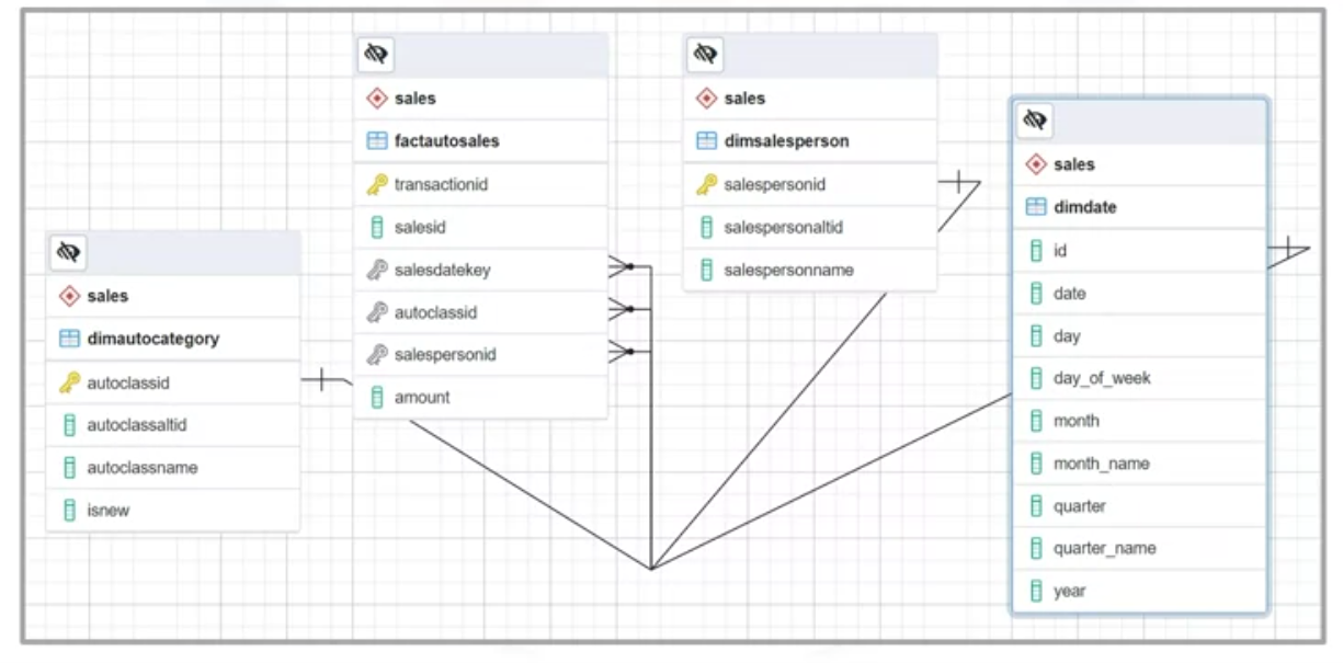
• You start a PostgreSQL session and generate an entity relationship diagram, or ERD, which represents the “Sales” star schema implemented within the ShinyAutoSales data warehouse, “sasDW.”
• Then, you locate the central fact table named “fact auto sales.” This table contains the “amount” column, which is the measure you need.
• You also spot the three foreign keys in the sales fact table: “sales date key,” “auto class ID,” and “salesperson ID.” These keys link respectively to:
• The “Date dimension table,” which contains dates and related values such as the day of the week, month name, and quarter.
• The “Auto category dimension table,” which includes the “auto class name,” and the Boolean “is new” column, and finally,
• the “Salesperson dimension table,” which contains the “salesperson’s name.”

In this example, you are using PostgreSQL. Let’s assume you already started up the terminal-based front-end to PostgreSQL, “P S Q L,” and connected to the “S A S D W” data warehouse.

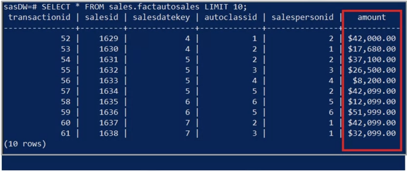
• Notice the command prompt contains the name of the data warehouse you are connected to, “S A S D W.”
• Starting with the auto sales fact table, you’ll enter the SQL statement “select star from sales dot fact auto sales limit 10” to display its first 10 rows.
• Here, you see the dollar amounts for individual auto sales, but the remaining columns are primary and foreign keys, which don’t have any direct meaning for you yet.
• However, you notice that the sales ID values are sequential, but the numbering starts at 1,629 instead of 1.
• That’s because ShinyAutoSales has provided you with access to a windowed subset of their data.

Next, you query the auto category dimension table.

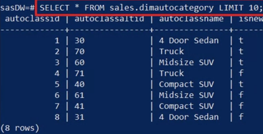
• Now, you can see meaningful names for various automobile classes, such as truck and compact SUVs.
• You notice duplicate entries for the truck class and wonder why they exist.
• When you look more closely, you realize the duplicate entries exist because of the distinct subclasses for new and used trucks.

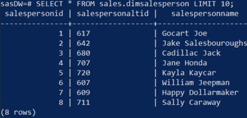
Similarly, you generate a view for the salesperson dimension table and find eight distinct salesperson names, including “Gocart Joe” and “Jane Honda.” So far, so good!

Finally, you view the date dimension table.

• You notice the dates only go back to January 1, 2021.
• Your contact at Shiny Auto Sales informs you that she will provide you with more data later and that for now, you can work with a smaller data set while you develop your queries.
• The date table contains potentially useful date elements such as the day of the week, month name, and quarter name.
• At this stage, it would be more convenient to have a table of data that contains the dimensions you need with human interpretable columns, rather than just keys.
• Essentially, you want to create a denormalized view of the data by joining the dimensions back to the fact of interest.

You proceed by selecting the “date,” “auto class name,” “is new,” “salesperson name,” and “amount” columns from their tables, and joining each dimension onto the “amount” fact using an inner join on the corresponding keys.

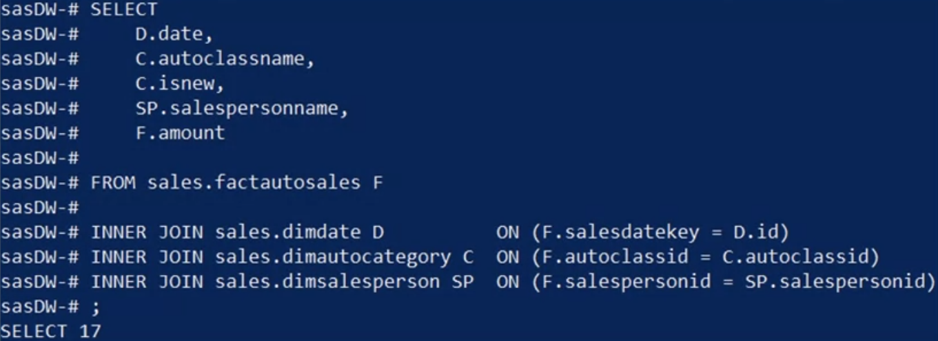
Next, why not capture the view as a materialized view called “Denormalized sales” or “D N sales” for short? Then you can reuse the materialized view for different queries without having to recreate your work.

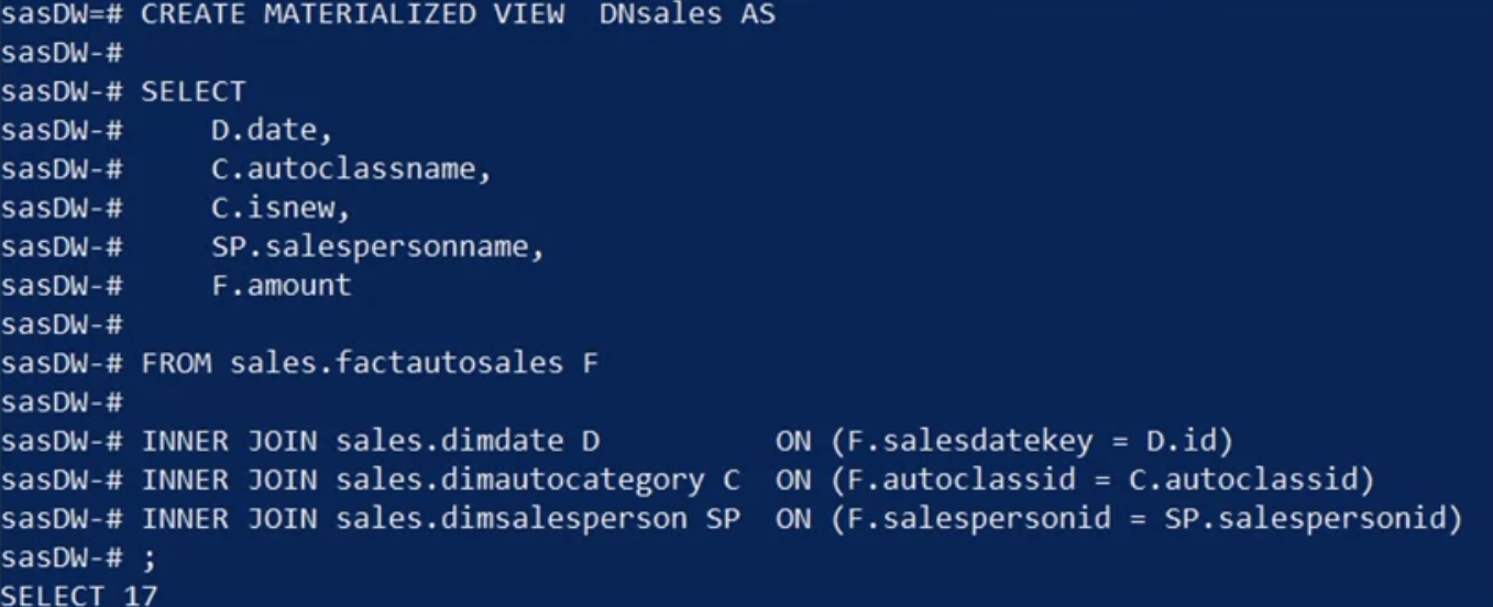
• You accomplish this task using the clause “CREATE MATERIALIZED VIEW D N sales AS,” followed by the same query you used to generate the denormalized view.

View the data :Type “Select star from D N sales, LIMIT 10” to display your resulting materialized view.

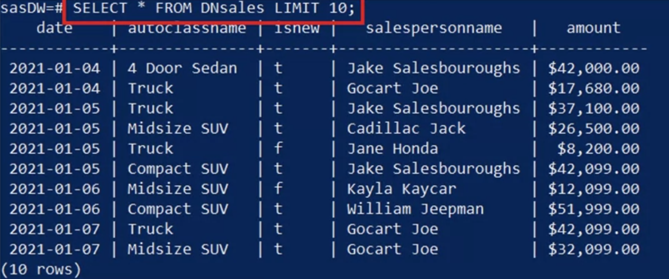
• Now you have a tidy, human-readable, time-series of sales data available for further analysis.
• For example, you can see that “Cadillac Jack” sold a new midsize SUV on January 5 for $26,500.

Cube

Next, you want to apply CUBE and ROLLUP operations to your denormalized, materialized view. Let’s see the CUBE results.

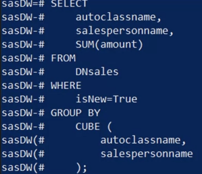
• Here, you select the “auto class name,” “salesperson name,” and the “sum of the sales amounts”
• from “D N sales,” where “is new” is set to “true.”
• Finally, group the generated cube by the “auto class name” and “salesperson name.”
• The output looks like this:

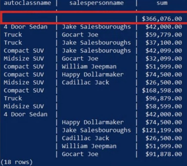
• The first row has no entries in the dimensions columns, which means ‘all.’ Thus, the value of $366,076 represents the total sales for all new cars.
• The next block of records has both dimension columns populated. So, for instance,
• you can read the total sales of new midsize SUVs by “Gocart Joe,” which is $32,099.
• Similarly, the last two blocks summarize “new auto sales” by class, and by salesperson.

Rollup

Next, you apply a ROLLUP instead of a CUBE operation. You decide to keep the query the same as the previous query, except that you replace CUBE with ROLLUP.

Here’s what the resulting view looks like now.

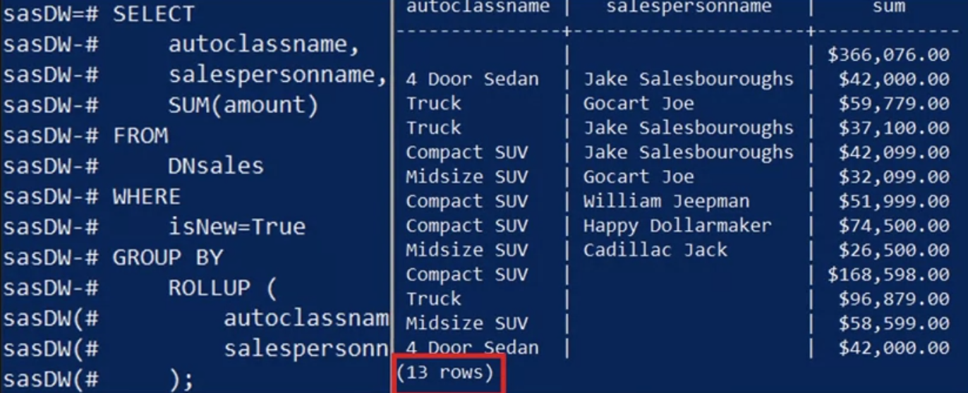
• You have five fewer rows with the ROLLUP result than CUBE, resulting in 13 rows instead of 18 rows.
• The only difference in this result is that you don’t have the “total sale amounts by salesperson” summary.

While CUBE generates all possible permutations of the “GROUP BY” columns, ROLLUP only looks at the single permutation defined by the columns’ order listed in the ROLLUP call.

Example

---

In this example we’ll go over the following:

• Grouping sets
• Rollup
• Cube
• Materialized Views

GROUPING SETS, CUBE, and ROLLUP allow us to easily create subtotals and grand totals in a variety of ways. All these operators are used along with the GROUP BY operator.

GROUPING SETS operator allows us to group data in a number of different ways in a single SELECT statement.

The ROLLUP operator is used to create subtotals and grand totals for a set of columns. The summarized totals are created based on the columns passed to the ROLLUP operator.

The CUBE operator produces subtotals and grand totals. In addition, it produces subtotals and grand totals for every permutation of the columns provided to the CUBE operator.

• Launch a PostgreSQL instance
• Open pgAdmin

Grouping Sets

Create a grouping set for three columns labeled year, category, and sum of billedamount, run the sql statement below.

select year,category, sum(billedamount) as totalbilledamount
from "FactBilling"
left join "DimCustomer"
on "FactBilling".customerid = "DimCustomer".customerid
left join "DimMonth"
on "FactBilling".monthid="DimMonth".monthid
group by grouping sets(year,category);

Rollup

To create a rollup using the three columns year, category and sum of billedamount, run the sql statement below.

select year,category, sum(billedamount) as totalbilledamount
from "FactBilling"
left join "DimCustomer"
on "FactBilling".customerid = "DimCustomer".customerid
left join "DimMonth"
on "FactBilling".monthid="DimMonth".monthid
group by rollup(year,category)
order by year, category;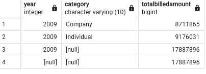

Cube

To create a cube using the three columns labeled year, category, and sum of billedamount, run the sql statement below.

select year,category, sum(billedamount) as totalbilledamount
from "FactBilling"
left join "DimCustomer"
on "FactBilling".customerid = "DimCustomer".customerid
left join "DimMonth"
on "FactBilling".monthid="DimMonth".monthid
group by cube(year,category)
order by year, category;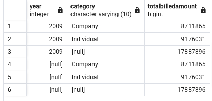

Materialized View

n pgAdmin we can implement materialized views using Materialized Query Tables.

Step 1: Create the Materialized views

Execute the sql statement below to create an Materialized views named countrystats.

CREATE MATERIALIZED VIEW countrystats (country, year, totalbilledamount) AS
(select country, year, sum(billedamount)
from "FactBilling"
left join "DimCustomer"
on "FactBilling".customerid = "DimCustomer".customerid
left join "DimMonth"
on "FactBilling".monthid="DimMonth".monthid
group by country,year);

# RESPONSE
Query returned successfully in 150 msec.

The above command creates an Materialized views named countrystats that has 3 columns.

• Country
• Year
• totalbilledamount

The Materialized views is essentially the result of the below query, which gives you the year, quartername and the sum of billed amount grouped by year and quartername.

select year, quartername, sum(billedamount) as totalbilledamount
from "FactBilling"
left join "DimCustomer"
on "FactBilling".customerid = "DimCustomer".customerid
left join "DimMonth"
on "FactBilling".monthid="DimMonth".monthid
group by grouping sets(year, quartername);

Step 2: Populate/refresh data into the Materialized views.

Execute the sql statement below to populate the Materialized views countrystats.

REFRESH MATERIALIZED VIEW countrystats;

# RESPONSE
Query returned successfully in 194 msec.

Step 3: Query the Materialized views.

Once an Materialized views is refreshed, you can query it. Execute the sql statement below to query the Materialized views countrystats.

select * from countrystats;

# OUTPUT is 129 rows some of which are shown below

Grouping Set

Create a grouping set for the columns year, quartername, sum(billedamount).

select year, quartername, sum(billedamount) as totalbilledamount
from "FactBilling"
left join "DimCustomer"
on "FactBilling".customerid = "DimCustomer".customerid
left join "DimMonth"
on "FactBilling".monthid="DimMonth".monthid
group by grouping sets(year, quartername);

Rollup

Create a rollup for columns country, category, sum(billedamount)

SELECT country, category, SUM(billedamount) AS totalbilledamount
FROM "FactBilling"
LEFT JOIN "DimCustomer"
ON "FactBilling".customerid = "DimCustomer".customerid
LEFT JOIN "DimMonth"
ON "FactBilling".monthid = "DimMonth".monthid
GROUP BY ROLLUP(country, category)
ORDER BY country, category;

# OUTPUT is 331 rows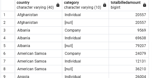

Cube

Create a cube for year, country, category, sum(billedamount)

SELECT year, country, category, SUM(billedamount) AS totalbilledamount
FROM "FactBilling"
LEFT JOIN "DimCustomer" 
ON "FactBilling".customerid = "DimCustomer".customerid
LEFT JOIN "DimMonth" 
ON "FactBilling".monthid = "DimMonth".monthid
GROUP BY CUBE(year, country, category);

# OUTPUT is 666 rows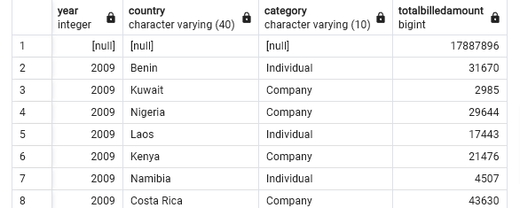

Materialized View

Create an Materialized views named average_billamount with columns year, quarter, category, country, average_bill_amount.

CREATE MATERIALIZED VIEW average_billamount (year,quarter,category,country, average_bill_amount) AS
    (select   year,quarter,category,country, avg(billedamount) as average_bill_amount
    from "FactBilling"
    left join  "DimCustomer"
    on "FactBilling".customerid =  "DimCustomer".customerid
    left join "DimMonth"
    on "FactBilling".monthid="DimMonth".monthid
    group by year,quarter,category,country
    );

Refresh

refresh MATERIALIZED VIEW average_billamount;

Query the View

select * from average_billamount;

# OUTPUT is 391 rows