Cubes Rollups & Views
Data Cube
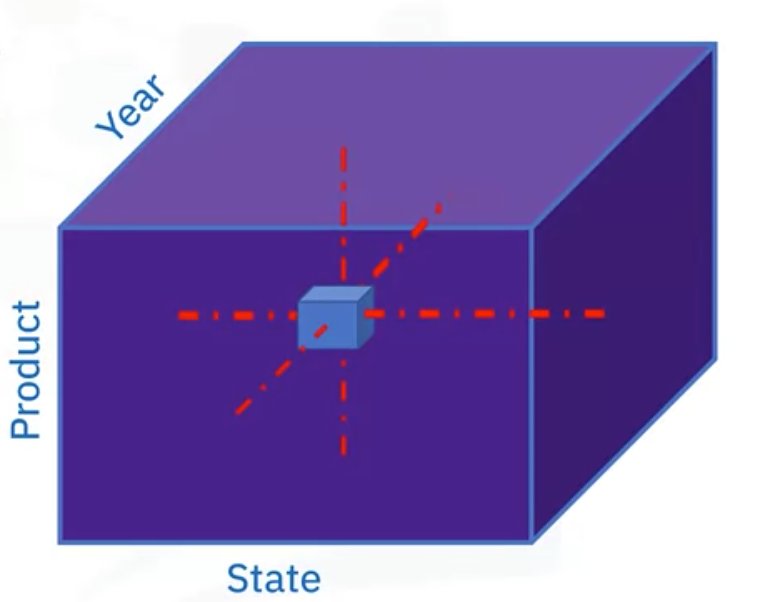
Let’s use an example to illustrate the concept of a data cube. Here is a cube generated from
- An imaginary star schema for a Sales OLAP (online analytical processing system).
- The coordinates of the cube are defined by a set of dimensions, which are selected from the star schema.
- In this illustration, we are only showing three dimensions, but data cubes can have many dimensions.
- We have the Product categories corresponding to the items sold,
- the State or Province the items were sold from, and
- the Year these products were sold in.
- The cells of the cube are defined by a fact of interest from the schema, which could be something like “total sales in thousands of dollars.” Here the “243” indicates “243 thousand dollars” for some given Product, State, and Year combination.
There are many operations you can perform on data cubes, such as
- slicing
- dicing
- drilling up and down
- pivoting and
- rolling up
Slicing
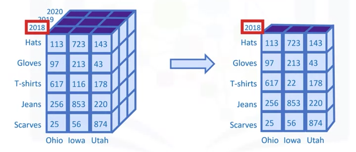
Slicing a data cube involves selecting a single member from a dimension, which yields a data cube that has one dimension less than the original.
For example, you can slice this sales cube by selecting only the year 2018 from the year dimension, allowing you to analyze sales totals for all sales states and all products for the year 2018.
Dicing
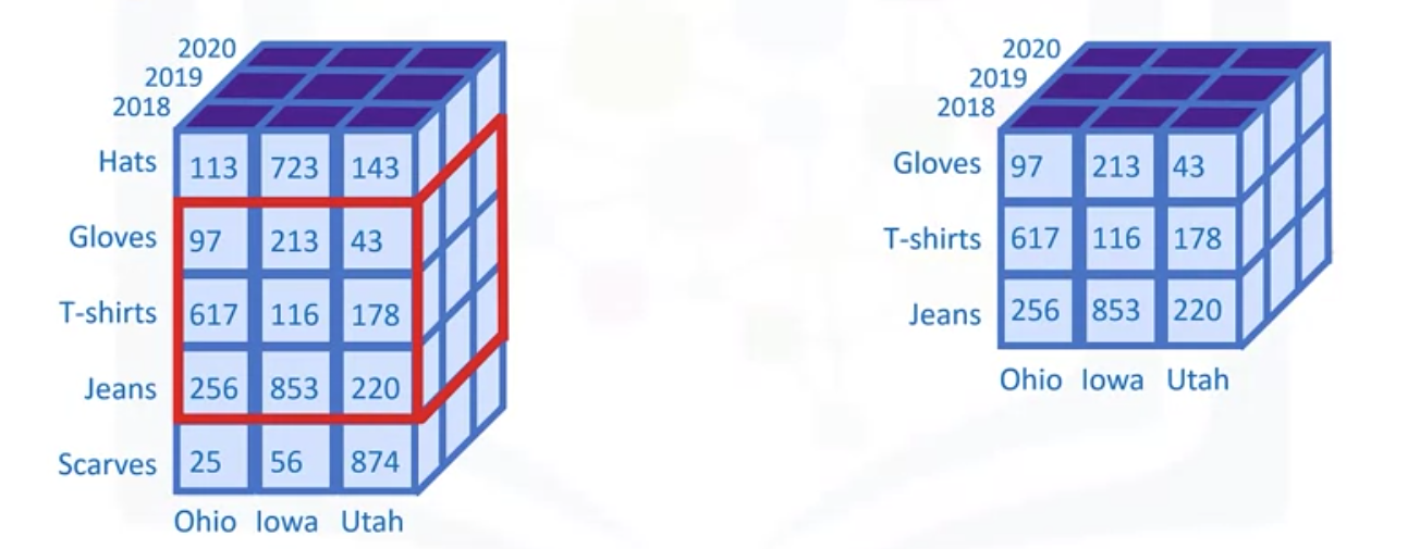
Similarly, dicing a cube involves selecting a subset of values from a dimension, effectively shrinking it.
For example, you can dice this sales cube by selecting only “Gloves”, “T-shirts”, and “Jeans” from the Product-Type dimension, allowing you to restrict your view to just those product types.
Drilling
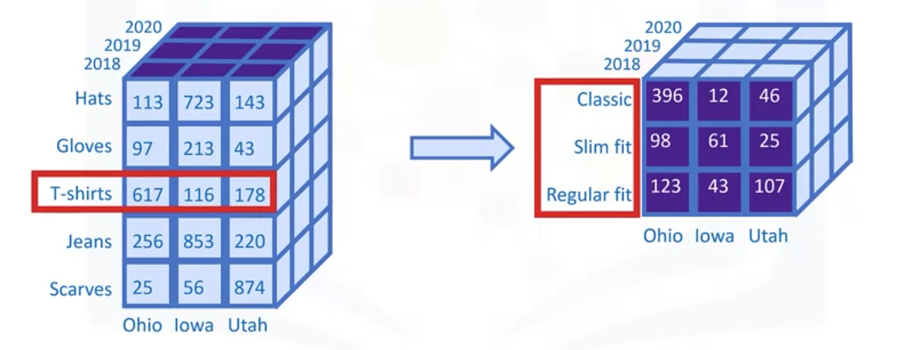
In snowflake schema, you will find hierarchies, or subcategories within some of your dimensions that you can drill into. Thus, for example, you can “drill down” into a particular member of the “Product category” dimension, such as “T-shirts,” resulting in this view, which may include more specific “product groups” such as “Classic,” “Slim fit,” and “Regular fit.”
Drilling up is just the reverse process, which would take you back to the original data cube.
Pivoting
Pivoting data cubes is straightforward. It involves a rotation of the data cube.
In this case, the year and product dimensions have been interchanged, while the State dimension has been fixed “as is.”
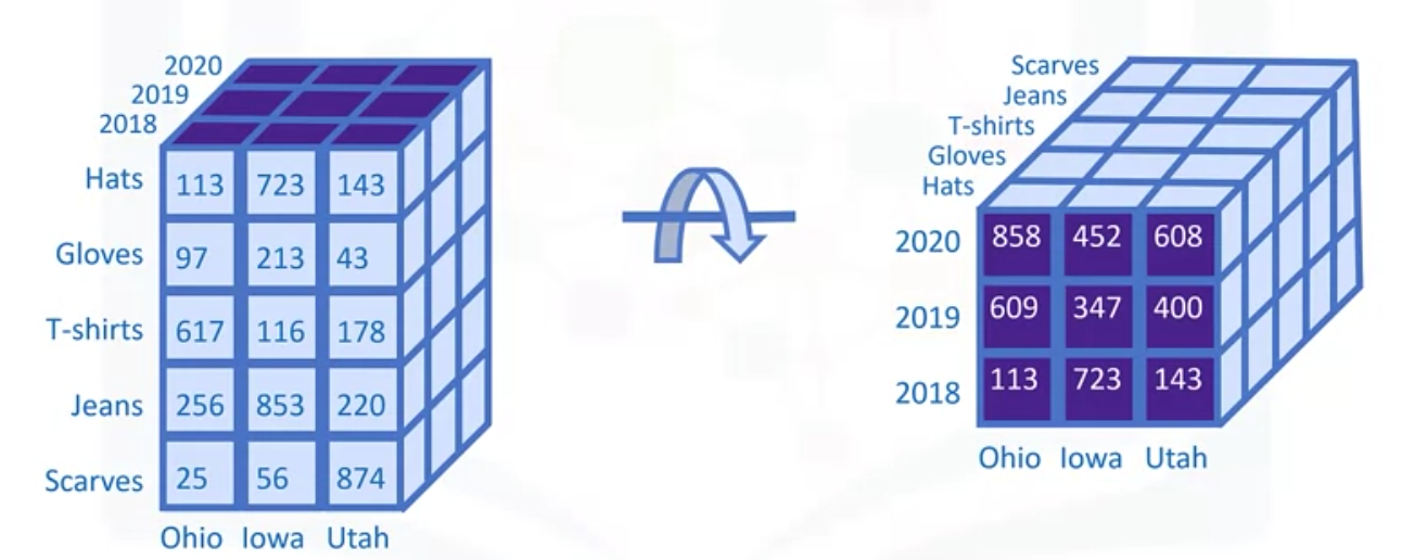
Pivoting doesn’t change its information content; it just changes the point of view you may choose to analyze it from.
Roll Up
Rolling up means summarizing along a dimension. You can roll up a dimension by applying aggregations, such as COUNT, MIN, MAX, SUM, and AVERAGE.
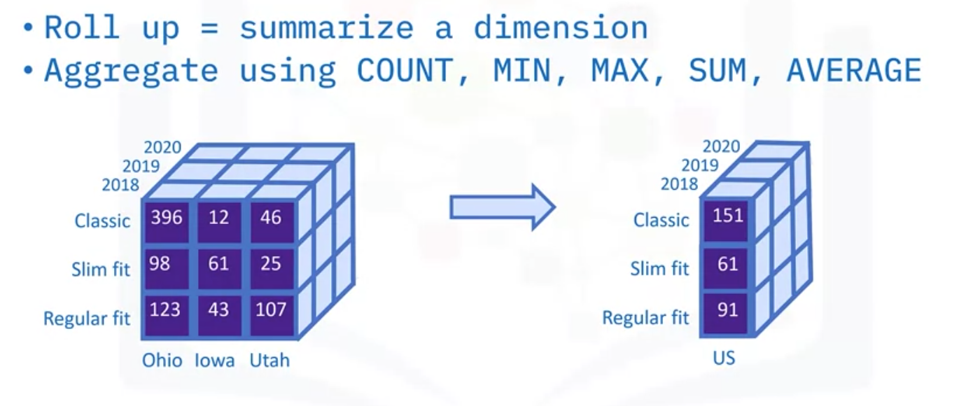
For example, you could calculate the average selling price of Classic, Slim fit, and Regularfit T-shirts by summing horizontally over the three US states and dividing by three.
Materialized View
A “materialized view” is essentially a local, read-only copy, or snapshot, of theresults of a query. They can be used to replicate data, for example to be used in a staging database as part of an ETL process, or to pre-compute and cache expensive queries, such as joins or aggregations, for use in data analytics environments.
- Materialized views also have options for automatically refreshing the data, thus keeping your queryup-to-date.
- Because materialized views can be queried, you can safely work with them without worrying about affecting the source database.
- Materialized Views can be set up to have different refresh options, such as:
- Never: they are only populated when created, which is useful if the data seldom changes.
- Upon request: manually refresh, for example, after changes to the data have been made,
- or scheduled refresh, for example, after daily data loads.
- Immediately: automatically refresh after every statement.
Oracle Example
Let’s look at an example: Here is how you might create a materialized view in Oracle using SQL statements.

- Start by creating and naming a “materialized view” object called MY_MAT_VIEW
- Specify the refresh type as fast, which means “incrementally refresh the data”.
- Specify today as the start date, and
- Refresh the view every day.
- The final statement selects all data from my_table_name
PostgreSQL Example
Here is how you might create a materialized view in PostgreSQL to replicate a table.

- Start by creating a “materialized view” object called MY_MAT_VIEW
- Specify some parameters,
- Specify the source tablespace, say tablespace_name, and
- Select all rows and columns from table_name
In PostgreSQL you can only refresh materialized views manually, using the “refresh materialview” command.
Db2 Example
In Db2, materialized views are called MQTs, which stands for “materialized query tables.”

Here’s an example, from IBM’s online documentation, of creating a system-maintained “immediate refresh” MQT.
- The table, which is named “emp,” is based on the underlying tables: “Employee” and “Department” from the “Sample” database.
- The table will be created according to the query formed by these SQL statements, which
- selects columns from both tables.
- The “data initially deferred” clause means that data will not be inserted into the table as part of the “create table” statement, while
- the “refresh immediate” clause specifies that the query should refresh automatically.
- The “immediate checked” clause specifies that the data is to be checked against the MQT’s defining query and refreshed.
- Lastly, the “not incremental” clause specifies that integrity checking is to be done on the whole table.

A query executed against the “emp” materialized query table shows that it is fully populated with data.